Prior shift, bag by bag#

Quantification lives or dies by prior-probability shift: the class distribution \(P(y)\) changes between bags while the class-conditional feature distribution \(P(x \mid y)\) stays the same. With make_quantification you can dial in exactly the prevalences you want by passing an explicit array of vectors, then watch the clusters keep their shape while their balance shifts.

import matplotlib.pyplot as plt

from mlquantify.datasets import make_quantification

# One bag per target prevalence — same population, different class balance.
targets = [[0.9, 0.1], [0.7, 0.3], [0.5, 0.5], [0.3, 0.7], [0.1, 0.9]]
Xs, ys, prevs = make_quantification(
    prevalence=targets, batch_size=500,
    n_features=2, n_redundant=0, class_sep=1.6, random_state=0,
)

fig, axes = plt.subplots(1, 5, figsize=(15, 3.3), sharex=True, sharey=True)
for ax, X, y, p in zip(axes, Xs, ys, prevs):
    for k, color in enumerate(["#2a9d8f", "#e76f51"]):
        mask = y == k
        ax.scatter(X[mask, 0], X[mask, 1], s=8, alpha=0.6, color=color)
    ax.set_title(f"class 1 = {p[1]:.0%}")
    ax.set_xticks([])
    ax.set_yticks([])
fig.suptitle("Same clusters, shifting prevalence — prior-probability shift", y=1.02)
fig.tight_layout()

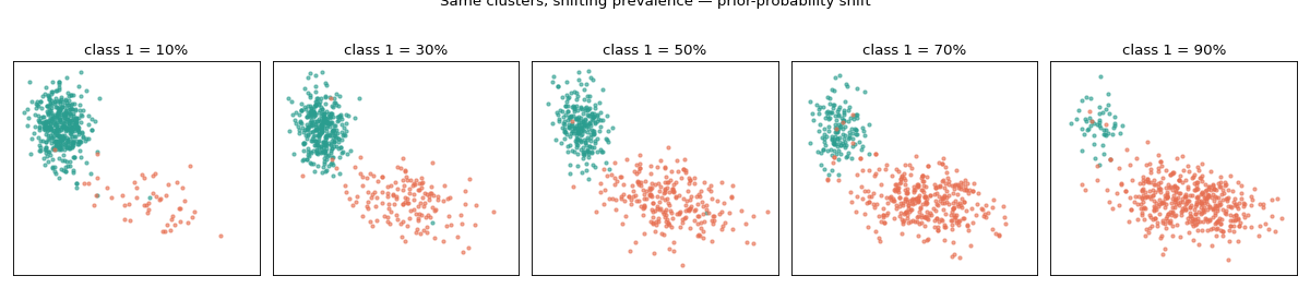
From left to right the orange class grows from 10% to 90% of the bag, yet each class always falls in the same region of feature space. That is precisely the regime quantifiers are built for — and precisely where a plain classifier’s count drifts off, because its error rates were learned at a different balance.

Pass prevalence="uniform" instead of an explicit list to draw the prevalences randomly across the whole simplex; see Controlling prevalence variability across bags.