Controlling prevalence variability across bags#

The prevalence argument (and, for the Dirichlet, concentration) decides how each bag’s class balance is drawn — i.e. how much the prevalence varies from bag to bag. This is the knob that turns make_quantification into the different evaluation protocols. The figure draws the distribution of the positive-class prevalence over many bags for each strategy.

import numpy as np
import matplotlib.pyplot as plt

from mlquantify.datasets import make_quantification

def positive_prevalences(**kwargs):
    _, _, prevs = make_quantification(
        n_batches=400, batch_size=200, n_features=2, n_redundant=0,
        random_state=0, **kwargs
    )
    return prevs[:, 1]

panels = [
    ("uniform — full range of shifts",
     dict(prevalence="uniform")),
    ("grid — even sweep (APP)",
     dict(prevalence="grid", n_prevalences=21)),
    ("natural — around weights=[0.6, 0.4]",
     dict(prevalence="natural", weights=[0.6, 0.4])),
    ("dirichlet near 0.7, concentration=200 (tight)",
     dict(prevalence="dirichlet", target_prevalence=[0.3, 0.7], concentration=200)),
    ("dirichlet near 0.7, concentration=8 (loose)",
     dict(prevalence="dirichlet", target_prevalence=[0.3, 0.7], concentration=8)),
]
colors = ["#264653", "#2a9d8f", "#e9c46a", "#e76f51", "#9b5de5"]

fig, axes = plt.subplots(len(panels), 1, figsize=(7, 8.5), sharex=True)
bins = np.linspace(0, 1, 31)
for ax, (title, kwargs), color in zip(axes, panels, colors):
    ax.hist(positive_prevalences(**kwargs), bins=bins, color=color, alpha=0.85)
    ax.set_title(title, fontsize="small")
    ax.set_yticks([])
axes[-1].set_xlabel("Positive-class prevalence of the bag")
fig.suptitle("How `prevalence` and `concentration` shape bag-to-bag variability")
fig.tight_layout()

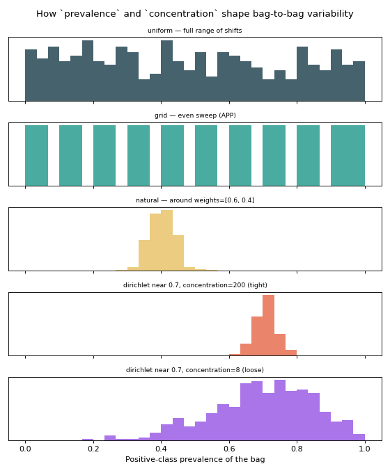
../_images/plot_synthetic_prevalence-1.png

Reading top to bottom: "uniform" spreads bags across the whole range (maximum shift), "grid" places them on regular points, "natural" clusters them tightly around the population prior, and the two Dirichlet panels show the same target of 0.70 with very different spreads — high concentration pins bags to the target, low concentration lets them wander. That single parameter is how you go from “test everywhere” to “test near a realistic operating point”.