Why counting fails under prior shift#

The central problem of quantification is prior-probability shift: the test class distribution differs from the training one. Plain Classify & Count (CC) simply counts the labels its classifier predicts, so it inherits the classifier’s misclassification rates and becomes biased as the test prevalence moves away from training.

ACC (Adjusted Classify & Count) corrects exactly this bias using the classifier’s true- and false-positive rates estimated on training data. The plot below sweeps the test prevalence across the full range and tracks what each method predicts.

import numpy as np
import matplotlib.pyplot as plt
from sklearn.datasets import make_classification
from sklearn.linear_model import LogisticRegression
from sklearn.model_selection import train_test_split

from mlquantify.counting import CC, ACC

X, y = make_classification(
    n_samples=6000, n_features=20, weights=[0.5, 0.5], random_state=1,
)
X_tr, X_pool, y_tr, y_pool = train_test_split(
    X, y, test_size=0.6, stratify=y, random_state=1,
)

cc = CC(LogisticRegression(max_iter=1000)).fit(X_tr, y_tr)
acc = ACC(LogisticRegression(max_iter=1000)).fit(X_tr, y_tr)

pos = np.where(y_pool == 1)[0]
neg = np.where(y_pool == 0)[0]
rng = np.random.default_rng(0)

target_prev = np.linspace(0.05, 0.95, 19)
cc_pred, acc_pred = [], []
for p in target_prev:
    n = 500
    n_pos = int(round(p * n))
    idx = np.concatenate([
        rng.choice(pos, n_pos, replace=True),
        rng.choice(neg, n - n_pos, replace=True),
    ])
    cc_pred.append(cc.predict(X_pool[idx])[1])
    acc_pred.append(acc.predict(X_pool[idx])[1])

fig, ax = plt.subplots(figsize=(6, 5.5))
ax.plot([0, 1], [0, 1], "k--", lw=1, label="ideal")
ax.plot(target_prev, cc_pred, "o-", color="#e76f51", label="CC (biased)")
ax.plot(target_prev, acc_pred, "s-", color="#2a9d8f", label="ACC (adjusted)")
ax.set_xlabel("True positive-class prevalence")
ax.set_ylabel("Predicted positive-class prevalence")
ax.set_title("CC drifts off the diagonal; ACC tracks it")
ax.set_aspect("equal")
ax.legend(loc="upper left")
fig.tight_layout()

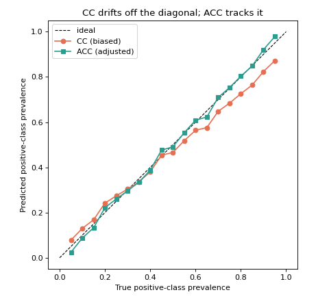
CC systematically pulls its estimate toward the training prevalence (the curve flattens away from the diagonal), while ACC stays close to the ideal line. This gap is the reason the rest of the library exists.