Distribution matching, step by step#

Distribution-matching quantifiers such as HDy and DyS estimate prevalence by a simple idea: the histogram of classifier scores on the test set should equal the prevalence-weighted mixture of the class-conditional score histograms learned on training. The quantifier searches for the positive-class prevalence \(\alpha\) whose mixture best matches the observed test histogram.

This example reconstructs that mechanism with plain matplotlib so you can see exactly what is being matched. We build the two class-conditional histograms, the observed test histogram, and the best-fit mixture found by sweeping \(\alpha\).

import numpy as np
import matplotlib.pyplot as plt
from sklearn.datasets import make_classification
from sklearn.linear_model import LogisticRegression
from sklearn.model_selection import train_test_split

rng = np.random.default_rng(0)
X, y = make_classification(
    n_samples=6000, n_features=20, weights=[0.5, 0.5], random_state=0,
)
X_tr, X_te, y_tr, y_te = train_test_split(
    X, y, test_size=0.5, random_state=0,
)

clf = LogisticRegression(max_iter=1000).fit(X_tr, y_tr)

bins = np.linspace(0, 1, 11)
def hist(scores):
    h, _ = np.histogram(scores, bins=bins, density=False)
    return h / h.sum()

s_tr = clf.predict_proba(X_tr)[:, 1]
h_neg = hist(s_tr[y_tr == 0])            # class-conditional histograms
h_pos = hist(s_tr[y_tr == 1])

# Build a test sample with ~70% positives and histogram its scores.
pos = np.where(y_te == 1)[0]
neg = np.where(y_te == 0)[0]
true_prev = 0.70
n = 800
idx = np.concatenate([
    rng.choice(pos, int(true_prev * n), replace=True),
    rng.choice(neg, n - int(true_prev * n), replace=True),
])
h_test = hist(clf.predict_proba(X_te[idx])[:, 1])

# Sweep alpha and pick the mixture closest to the test histogram (L2).
alphas = np.linspace(0, 1, 201)
losses = [np.sum(((1 - a) * h_neg + a * h_pos - h_test) ** 2) for a in alphas]
a_hat = alphas[int(np.argmin(losses))]
mixture = (1 - a_hat) * h_neg + a_hat * h_pos

centers = (bins[:-1] + bins[1:]) / 2
fig, (ax1, ax2) = plt.subplots(1, 2, figsize=(11, 4.5))

width = (bins[1] - bins[0]) * 0.9
ax1.bar(centers, h_test, width=width, color="#bdbdbd", label="test histogram")
ax1.step(centers, mixture, where="mid", color="#e63946", lw=2,
         label=f"best-fit mixture ($\\hat\\alpha$={a_hat:.2f})")
ax1.step(centers, h_pos, where="mid", color="#457b9d", ls="--",
         label="class-conditional: positive")
ax1.step(centers, h_neg, where="mid", color="#2a9d8f", ls="--",
         label="class-conditional: negative")
ax1.set_xlabel("Classifier score  P(y=1)")
ax1.set_ylabel("Frequency")
ax1.set_title("What is being matched")
ax1.legend(fontsize="small")

ax2.plot(alphas, losses, color="#264653")
ax2.axvline(a_hat, color="#e63946", ls=":", label=f"$\\hat\\alpha$={a_hat:.2f}")
ax2.axvline(true_prev, color="k", ls="--", lw=1, label=f"true={true_prev:.2f}")
ax2.set_xlabel(r"Candidate positive prevalence  $\alpha$")
ax2.set_ylabel("Histogram mismatch (L2)")
ax2.set_title("The objective being minimised")
ax2.legend()
fig.tight_layout()

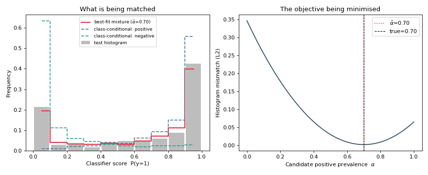
../_images/plot_distribution_matching-1.png

The left panel shows the test histogram with the matched mixture sitting almost on top of it; the right panel shows the matching loss as a function of \(\alpha\), with its minimum landing close to the true prevalence. Real methods differ mainly in the distance they minimise — Hellinger for HDy, Topsøe / a tunable mixture for DyS — and in how finely they search.