Benchmarking quantifiers on synthetic bags#

With a synthetic population we know every bag’s true prevalence, so we can score quantifiers exactly. The recipe: ask make_quantification for a fixed training sample plus many shifted test bags, fit each quantifier once on the training sample, predict every bag, and plot predicted vs. true prevalence.

To make it a realistic stress test we use a harder, three-class problem — 20 features (mostly noise), low class separation, 5% label noise — and stack all three shifts: a full prior sweep plus a small dose of covariate and concept shift (low covariate_scale / concept_strength) for extra variability.

import numpy as np
import matplotlib.pyplot as plt
from sklearn.linear_model import LogisticRegression

from mlquantify import set_config
from mlquantify.datasets import make_quantification
from mlquantify.counting import CC, ACC
from mlquantify.likelihood import EMQ
from mlquantify.matching import DyS
from mlquantify.visualization import DiagonalDisplay

# Make every quantifier return prevalences as a plain, class-ordered array.
set_config(prevalence_return_type="array")

Xtr, ytr, Xs, ys, prevs = make_quantification(
    n_batches=200, batch_size=200, return_train=True, n_classes=3,
    train_prevalence=[1 / 3, 1 / 3, 1 / 3],
    # mostly prior shift, with a little covariate + concept for realism
    shift_type=["prior", "covariate", "concept"], prevalence="uniform",
    covariate_scale=0.3, concept_strength=0.2,
    n_features=20, n_redundant=0, class_sep=0.6, flip_y=0.05, random_state=0,
)

methods = {
    "CC": CC(LogisticRegression(max_iter=1000)),
    "ACC": ACC(LogisticRegression(max_iter=1000)),
    "EMQ": EMQ(LogisticRegression(max_iter=1000)),
    "DyS": DyS(LogisticRegression(max_iter=1000)),
}

fig, axes = plt.subplots(2, 2, figsize=(9, 9))
for (name, q), ax in zip(methods.items(), axes.ravel()):
    q.fit(Xtr, ytr)
    pred = np.vstack([q.predict(Xb) for Xb in Xs])
    # DiagonalDisplay colour-codes the three classes automatically.
    DiagonalDisplay.from_predictions(prevs, pred, ax=ax, alpha=0.4, s=14)
    mae = float(np.mean(np.abs(pred - prevs)))
    ax.set_title(f"{name}  (MAE = {mae:.3f})")
fig.suptitle("3-class quantifiers under stacked shift (prior + a little covariate/concept)",
             y=0.99)
fig.tight_layout()

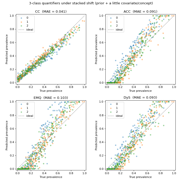
../_images/plot_synthetic_quantifiers-1.png

Each panel colour-codes the three classes, and the MAE in the title is computed directly from the returned prevs — no protocol bookkeeping. Compared with an easy, clean problem every cloud is visibly wider here: the harder population and the small dose of covariate/concept shift push the estimates off the diagonal. The extra shift — which breaks the pure prior-shift assumption — perturbs the adjustment-based methods (ACC, EMQ, DyS) the most, while plain CC stays comparatively tight, a reminder that the “best” method depends on the shift.

Dial covariate_scale / concept_strength up or down to control how far the bags wander, or drop them entirely (shift_type="prior") for a clean prior-shift benchmark.