EMQ and the EM prior correction#

EMQ (also known as SLD or the Saerens–Latinne–Decaestecker method) adjusts a classifier’s posteriors to a new test prevalence using Expectation-Maximisation. Starting from the training prior, it alternates between (E) re-scaling the posteriors by the current prevalence estimate and (M) averaging them into a new prevalence — repeating until the estimate stops moving.

The example below runs that exact loop by hand on a shifted test sample, recording the prevalence after every iteration so we can watch it converge from the (wrong) training prior to the true test prevalence.

import numpy as np
import matplotlib.pyplot as plt
from sklearn.datasets import make_classification
from sklearn.linear_model import LogisticRegression
from sklearn.model_selection import train_test_split

rng = np.random.default_rng(0)
X, y = make_classification(
    n_samples=6000, n_features=20, weights=[0.5, 0.5], random_state=0,
)
X_tr, X_te, y_tr, y_te = train_test_split(X, y, test_size=0.5, random_state=0)

clf = LogisticRegression(max_iter=1000).fit(X_tr, y_tr)
train_prior = np.array([(y_tr == 0).mean(), (y_tr == 1).mean()])

# A strongly positive test sample (true positive prevalence = 0.80).
pos = np.where(y_te == 1)[0]
neg = np.where(y_te == 0)[0]
true_prev = 0.80
n = 800
idx = np.concatenate([
    rng.choice(pos, int(true_prev * n), replace=True),
    rng.choice(neg, n - int(true_prev * n), replace=True),
])
Px = clf.predict_proba(X_te[idx])

# The EMQ fixed-point iteration (same update as mlquantify's EMQ.EM).
qs = train_prior.copy()
history = [qs[1]]
for _ in range(25):
    ratio = qs / train_prior
    ps = Px * ratio
    ps /= ps.sum(axis=1, keepdims=True)
    qs = ps.mean(axis=0)
    history.append(qs[1])

fig, ax = plt.subplots(figsize=(7, 4.5))
ax.plot(history, "o-", color="#2a9d8f", label="EMQ estimate")
ax.axhline(true_prev, color="k", ls="--", lw=1, label=f"true = {true_prev:.2f}")
ax.axhline(train_prior[1], color="#e76f51", ls=":", lw=1,
           label=f"training prior = {train_prior[1]:.2f}")
ax.set_xlabel("EM iteration")
ax.set_ylabel("Estimated positive prevalence")
ax.set_title("EMQ converges from the training prior to the true prevalence")
ax.set_ylim(0, 1)
ax.legend(loc="center right")
fig.tight_layout()

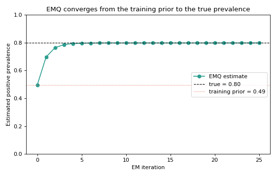
The estimate starts at the training prior (0.5, the wrong answer for this sample), then climbs and flattens out near the true 0.80 within a handful of iterations. In practice you never write this loop yourself — EMQ(...).predict does it for you — but seeing it unrolled makes the method’s behaviour concrete.