Confidence intervals and regions#

A prevalence estimate is more useful with an honest measure of its uncertainty. Bootstrapping the test sample — predicting on many resamples — turns a single point estimate into a distribution of estimates, from which we can read a confidence interval (binary) or a confidence region on the simplex (multiclass).

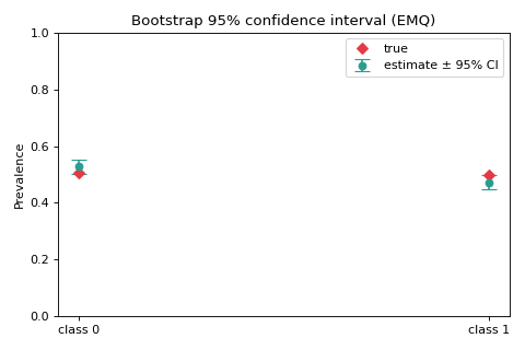
Binary: a bootstrap confidence interval#

We resample the test set, re-predict each time, and summarise the spread with a percentile interval via construct_confidence_region.

import numpy as np
import matplotlib.pyplot as plt
from sklearn.datasets import make_classification
from sklearn.linear_model import LogisticRegression
from sklearn.model_selection import train_test_split

from mlquantify.likelihood import EMQ
from mlquantify.confidence import construct_confidence_region

X, y = make_classification(
    n_samples=4000, n_features=20, weights=[0.5, 0.5], random_state=0,
)
X_tr, X_te, y_tr, y_te = train_test_split(X, y, test_size=0.5, random_state=0)

q = EMQ(LogisticRegression(max_iter=1000)).fit(X_tr, y_tr)

rng = np.random.default_rng(0)
boot = []
for _ in range(300):
    idx = rng.choice(len(X_te), len(X_te), replace=True)
    pred = q.predict(X_te[idx])
    boot.append([pred[c] for c in q.classes_])
boot = np.array(boot)

region = construct_confidence_region(
    boot, confidence_level=0.95, method="intervals",
)
low, high = region.get_region()
point = boot.mean(axis=0)
true = np.array([(y_te == c).mean() for c in q.classes_])

fig, ax = plt.subplots(figsize=(6, 4))
xpos = np.arange(len(q.classes_))
ax.errorbar(
    xpos, point, yerr=[point - low, high - point],
    fmt="o", capsize=6, color="#2a9d8f", label="estimate ± 95% CI",
)
ax.plot(xpos, true, "D", color="#e63946", label="true")
ax.set_xticks(xpos)
ax.set_xticklabels([f"class {c}" for c in q.classes_])
ax.set_ylabel("Prevalence")
ax.set_ylim(0, 1)
ax.set_title("Bootstrap 95% confidence interval (EMQ)")
ax.legend()
fig.tight_layout()

../_images/plot_confidence_regions-1.png

Three classes: a confidence region on the simplex#

With three classes the estimate lives on a 2-simplex, and the natural uncertainty summary is a confidence ellipse. ConfidenceRegionDisplay draws the bootstrap cloud and its ellipse directly.

import numpy as np
from sklearn.datasets import make_classification
from sklearn.linear_model import LogisticRegression
from sklearn.model_selection import train_test_split

from mlquantify.likelihood import EMQ
from mlquantify.visualization import ConfidenceRegionDisplay

X, y = make_classification(
    n_samples=4500, n_features=20, n_informative=6,
    n_classes=3, n_clusters_per_class=1, random_state=0,
)
X_tr, X_te, y_tr, y_te = train_test_split(X, y, test_size=0.5, random_state=0)

q = EMQ(LogisticRegression(max_iter=1000)).fit(X_tr, y_tr)

rng = np.random.default_rng(0)
boot = []
for _ in range(400):
    idx = rng.choice(len(X_te), len(X_te), replace=True)
    pred = q.predict(X_te[idx])
    boot.append([pred[c] for c in q.classes_])
boot = np.array(boot)
true = np.array([(y_te == c).mean() for c in q.classes_])

ConfidenceRegionDisplay.from_estimates(
    boot, confidence_level=0.95,
    class_names=["A", "B", "C"], true_prevalence=true,
    color="#1d3557", alpha=0.25,
)

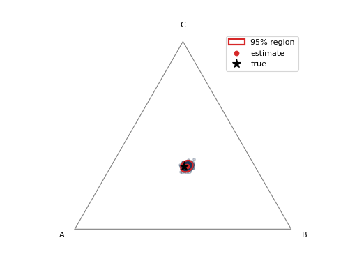
../_images/plot_confidence_regions-2.png

The ellipse shows both the size of the uncertainty (area) and its orientation (which classes trade off against each other). If the true point falls inside the 95% region, the quantifier’s uncertainty estimate is well-calibrated.