2.5. Adjusted Counting#
Adjusted counting methods correct the bias of naive counting by using what the classifier’s error rates reveal about the true class distribution. They are the oldest family of dedicated quantification methods (Forman, 2005) and remain strong baselines for binary problems.
Binary-only, multiclass via OvR
All methods on this page are fundamentally binary. When you apply them to a
dataset with more than two classes, mlquantify automatically decomposes
the problem into K one-vs-rest (OvR) binary subproblems and recombines
the results. Pass strategy='ovo' to use one-vs-one instead.
2.5.1. The Adjustment Formula#
All adjusted counting methods share the same core correction derived from the confusion matrix. Suppose a binary classifier has true positive rate TPR and false positive rate FPR (estimated on training data). If CC returns an observed positive proportion \(\hat{p}^{CC}\), the adjusted estimate is:
The methods below differ only in how they pick the threshold on the ROC curve at which TPR and FPR are read off. The formula itself is the same for all of them. (Forman, 2005, 2008)
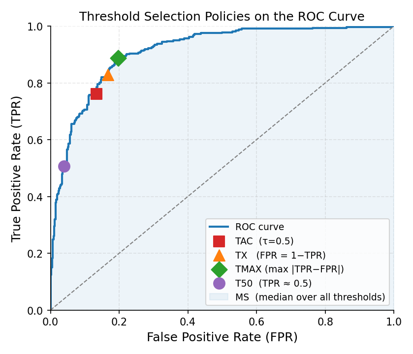
Each threshold-adjustment method picks a different operating point on the ROC curve. TAC uses τ=0.5 (red square); TX selects the symmetric crossing point (orange triangle); TMAX picks the point of maximum TPR−FPR separation (green diamond); T50 targets TPR≈0.5 (purple circle). MS sweeps the shaded area and takes the median.#
Why the formula works
Consider the population of test items. Each item can be truly positive or negative. The CC count can be decomposed as:
Solving for \(p(\oplus)\) gives the AC formula. The correction is exact when TPR and FPR are known; in practice they are estimated from cross-validated training predictions, so a small estimation error remains.
2.5.2. ACC — Adjusted Classify and Count (hard predictions)#
ACC applies the adjustment formula using the classifier’s argmax
(hard) predictions, rather than a soft-probability threshold. TPR and FPR
are computed by comparing the classifier’s hard labels against the true
training labels.
Why it exists: ACC is the “reference” adjusted-counting method described in Forman (2005). By deriving TPR/FPR from hard predictions it matches the behaviour expected from the theoretical derivation and avoids threshold selection entirely.
2.5.2.1. Parameters#
Parameter |
Default |
Explanation |
|---|---|---|
|
|
A classifier with |
|
|
Multiclass decomposition strategy ( |
|
|
Folds for cross-validating the confusion matrix. More folds → better TPR/FPR estimates but longer fitting. 5–10 is recommended. |
|
|
Use stratified folds to ensure rare classes appear in every fold.
Always leave |
|
|
Shuffle before splitting. Set |
|
|
Seed for reproducible splits. |
|
|
Parallel jobs for OvR/OvO decomposition. |
2.5.2.2. Examples#
from mlquantify.counting import ACC
from sklearn.linear_model import LogisticRegression
from sklearn.datasets import make_classification
from sklearn.model_selection import train_test_split

X, y = make_classification(n_samples=1000, weights=[0.8, 0.2],
                           random_state=42)
X_train, X_test, y_train, y_test = train_test_split(
    X, y, test_size=0.3, random_state=42)

q = ACC(LogisticRegression(), cv=5)
q.fit(X_train, y_train)
print(q.predict(X_test))
# {0: 0.79, 1: 0.21}
2.5.3. ThresholdAdjustment — Base Class for ROC-Threshold Methods#
ThresholdAdjustment is the abstract base for all ROC-based adjusted
counting methods. Subclasses implement get_best_threshold to select
the threshold at which to evaluate TPR and FPR. The adjustment formula is
then applied at that chosen point.
You can subclass it to implement custom threshold-selection policies:
from mlquantify.counting import ThresholdAdjustment
import numpy as np

class HalfTPR(ThresholdAdjustment):
    """Select the threshold where TPR ≈ 0.5."""
    def get_best_threshold(self, thresholds, tprs, fprs):
        idx = np.argmin(np.abs(tprs - 0.5))
        return thresholds[idx], tprs[idx], fprs[idx]
2.5.4. TAC — Threshold Adjusted Count (fixed threshold)#
TAC evaluates TPR and FPR at a fixed threshold (default 0.5)
and applies the AC formula at that single point.
Why it exists: TAC is the simplest threshold-adjustment method. It uses the natural decision boundary of the classifier without any search. It is often dominated by methods that pick a better threshold, but serves as a useful reference.
2.5.4.1. Parameters#
Parameter |
Default |
Explanation |
|---|---|---|
|
|
Probabilistic classifier ( |
|
|
The classification threshold at which TPR/FPR are evaluated. Change this when you know your classifier works better at a non-default cutoff (e.g. 0.3 for imbalanced classes). |
|
|
Folds for cross-validating soft scores used to build the ROC curve. |
|
|
See |
|
|
Multiclass decomposition. |
|
|
Parallel jobs for decomposition. |
2.5.4.2. Examples#
from mlquantify.counting import TAC
from sklearn.linear_model import LogisticRegression

q = TAC(LogisticRegression(), threshold=0.5)
q.fit(X_train, y_train)
print(q.predict(X_test))
# {0: 0.79, 1: 0.21}
2.5.5. TX — Threshold X (symmetric ROC point)#
TX selects the threshold where \(\text{FPR} = 1 - \text{TPR}\),
i.e., the intersection of the FPR curve and the (1 − TPR) curve. This
corresponds to the point on the ROC curve equidistant from both axes.
Why it exists: At this symmetric point the classifier makes a balanced tradeoff between false positives and false negatives, which tends to give a stable AC estimate. Forman (2005) found TX competitive across many benchmark tasks.
from mlquantify.counting import TX
from sklearn.linear_model import LogisticRegression

q = TX(LogisticRegression())
q.fit(X_train, y_train)
print(q.predict(X_test))
2.5.6. TMAX — Maximum TPR−FPR Separation#
TMAX selects the threshold that maximises \(|\text{TPR} - \text{FPR}|\),
which is the point of highest discriminative power on the ROC curve.
Why it exists: A large \(\text{TPR} - \text{FPR}\) gap makes the AC denominator large and keeps the adjusted estimate numerically stable. TMAX is useful when the classifier has a clear peak in discriminative power.
from mlquantify.counting import TMAX
from sklearn.linear_model import LogisticRegression

q = TMAX(LogisticRegression())
q.fit(X_train, y_train)
print(q.predict(X_test))
2.5.7. T50 — TPR ≈ 0.5 Threshold#
T50 selects the threshold where the true positive rate is closest
to 0.5, placing the operating point in the middle of the ROC curve.
Why it exists: Extreme thresholds (near 0 or 1 on the ROC) can yield unstable estimates when TPR or FPR is close to 0. T50 avoids both extremes, giving a conservative but robust estimate. Forman (2005) introduced it as an alternative to TX.
from mlquantify.counting import T50
from sklearn.linear_model import LogisticRegression

q = T50(LogisticRegression())
q.fit(X_train, y_train)
print(q.predict(X_test))
2.5.8. MS — Median Sweep#
MS applies the AC formula at every threshold on the ROC curve
and returns the median of all resulting prevalence estimates.
Why it exists: Any single-threshold method is sensitive to the exact threshold it picks. By sweeping all thresholds and taking the median, MS is robust to a bad individual threshold. Forman (2008) showed it is often the most accurate method across a wide range of test prevalences.
from mlquantify.counting import MS
from sklearn.linear_model import LogisticRegression

q = MS(LogisticRegression())
q.fit(X_train, y_train)
print(q.predict(X_test))
2.5.9. MS2 — Median Sweep with Constraint#
MS2 is a constrained variant of MS. It only uses
thresholds where \(|\text{TPR} - \text{FPR}| > 0.25\), discarding
regions of the ROC curve where the classifier is nearly non-discriminative
(and where the AC denominator is close to zero, causing numerical instability).
Why it exists: Thresholds where TPR ≈ FPR inflate the adjusted estimate wildly. MS2 filters them out before taking the median, making it more stable than MS on noisy classifiers. Forman (2008) introduced it as an improvement over plain MS.
2.5.9.1. Parameters#
Parameter |
Default |
Explanation |
|---|---|---|
|
|
Probabilistic classifier. |
|
|
Cross-validation folds for the soft score distribution. |
|
|
Stratified folds. |
|
|
Multiclass decomposition. |
|
|
Parallel jobs. |
from mlquantify.counting import MS2
from sklearn.linear_model import LogisticRegression

q = MS2(LogisticRegression())
q.fit(X_train, y_train)
print(q.predict(X_test))
2.5.10. Comparing Threshold-Adjustment Methods#
Method |
Threshold rule |
Strength |
Use when |
|---|---|---|---|
ACC |
Hard-prediction argmax |
Exact AC derivation; no threshold to choose |
You want the canonical AC method |
TAC |
Fixed \(\tau\) (default 0.5) |
Simplest; good when calibrated at 0.5 |
Classifier is calibrated at default threshold |
TX |
\(\text{FPR} = 1 - \text{TPR}\) |
Balanced operating point |
General-purpose binary quantification |
TMAX |
Max \(|\text{TPR} - \text{FPR}|\) |
Most stable denominator |
Classifier has a sharp discrimination peak |
T50 |
TPR closest to 0.5 |
Avoids extreme thresholds |
Unstable estimates at extreme thresholds |
MS |
Median over all thresholds |
Robust to threshold choice |
Default choice; works well on most tasks |
MS2 |
Median over \(|\text{TPR}-\text{FPR}|>0.25\) |
Stable on noisy classifiers |
Classifier has poor discrimination in parts of ROC |
Practical recommendation: Start with MS or MS2 — Forman (2008) showed they consistently outperform single-threshold methods. If you want the canonical ACC correction without ROC sweep, use ACC.
See also
Counting-Based Quantifiers for the simpler CC / PCC / GACC / GPACC family. Likelihood-Based Quantification for EMQ, which usually outperforms adjusted counting.
Adjusted Counting methods improve upon simple “counting” quantifiers by correcting bias using what is known about the classifier’s errors on the training set. They aim to produce better estimates of class prevalence (how frequent each class is in a dataset) even when training and test distributions differ.
see Counting-Based Quantifiers for an overview of the base counters for quantification.
This page focuses on threshold adjustment methods, which adjust the decision threshold of a classifier to optimize prevalence estimation. Examples include Adjusted Count (TAC) and its threshold selection policies (TX, TMAX, T50, MS, MS2).
2.5.11. Threshold Adjustment#
Threshold-based adjustment methods correct the bias of CC by using the classifier’s True Positive Rate (TPR) and False Positive Rate (FPR).
They are mainly used for binary quantification tasks.
Threshold Adjusted Count (TAC) Equation
- caption:
Corrected prevalence estimate using classifier error rates
The main idea is that by adjusting the observed rate of positive predictions, we can better approximate the real class distribution.
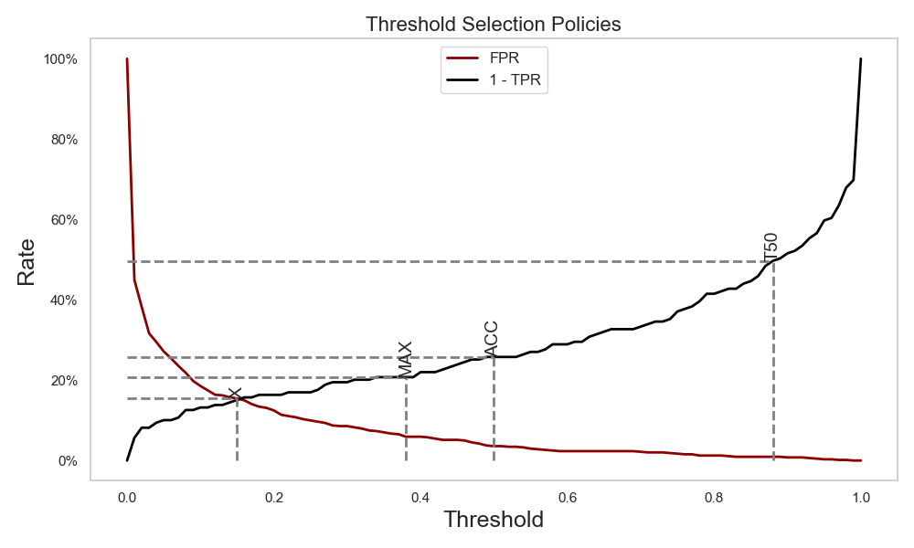
Comparison of different threshold selection policies showing FPR and 1-TPR curves with optimal thresholds for each method [Adapted from Forman (2008)]#
Different threshold methods vary in how they choose the classifier cutoff \(\tau\) for scores \(s(x)\) .
All these methods have their fit, predict and aggregate functions, similar to other aggregative quantifiers. However, they also include a specialized method: get_best_thresholds, which identifies the optimal threshold, given y and predicted probabilities. Here is an example of how to use the T50 method:
from mlquantify.counting import T50, evaluate_thresholds
from sklearn.linear_model import LogisticRegression

clf = LogisticRegression()

thresholds, tprs, fprs = evaluate_thresholds(
   y=y_test,
   probabilities=clf.predict_proba(X_test)[:, 1]) # binary proba

q = T50()
best_thr, best_tpr, best_fpr = q.get_best_thresholds(X_val, y_val)
print(f"Best threshold: {best_thr}, TPR: {best_tpr}, FPR: {best_fpr}")
Note
Threshold adjustment methods like TAC are primarily designed for binary classification tasks.