2.7. Distribution Matching

Distribution matching (DM) methods estimate prevalences without inverting a confusion matrix or re-weighting posteriors. Instead, they find the mixture proportion of class-conditional distributions that best reproduces the observed test distribution. This makes them highly versatile: they can handle non-standard classifiers, non-linear shift, and multiclass problems natively.

Core idea: During training, DM methods learn a representation \(r_c\) of each class’s distribution (a histogram, density, kernel mean, …). At test time, they find the prevalence vector \(\hat{p}\) such that the mixture

\[\sum_c \hat{p}(c) \cdot r_c \;\approx\; r_U\]

is as close as possible to the test representation \(r_U\), under some dissimilarity measure. This is solved as a constrained optimisation over the probability simplex.

mlquantify organises distribution matching into four representation families — histogram, density (KDE), kernel, and scores — all exposed through mlquantify.matching.

---

2.7.1. Histogram Methods

Histogram methods discretise the classifier’s score distribution into bins. They are the oldest DM family and remain competitive on binary problems.

Binary-only (unless noted)

Histogram methods are fundamentally binary. mlquantify applies OvR decomposition automatically for multiclass datasets.

2.7.1.1. DyS — Distribution y-Similarity

DyS (Maletzke et al., 2019) builds a histogram of classifier scores for each class from cross-validated predictions. At test time it searches for the mixture proportion \(\alpha \in [0,1]\) that minimises a dissimilarity measure between the test score histogram and the mixture of class histograms:

\[\hat{p}^{DyS}(\oplus) = \arg\min_{\alpha \in [0,1]} D\!\left( \alpha \cdot H_+ + (1-\alpha) \cdot H_- ,\; H_U \right)\]

Why it excels: DyS is a framework that separates the representation (histogram), the dissimilarity measure, and the solver. It can be configured with any distance and bin size. Maletzke et al. (2019) showed it beats threshold-adjustment methods and matches EMQ on many benchmarks.

2.7.1.2. Parameters

Parameter	Default	Explanation
estimator	None	Probabilistic classifier (predict_proba). Its cross-validated scores are used to build the class histograms.
bins_size	None	Number of histogram bins, or an array of bin counts to sweep. If None, a default logarithmic grid is used. Larger bins give a coarser representation (more stable but less expressive); smaller bins capture more detail but are noisier with limited training data.
distance	'topsoe'	Dissimilarity measure between histograms. Options: 'topsoe' (default) — Jensen–Shannon-like, recommended for DyS. 'hellinger' — square root of half the chi-squared distance. 'probsymm' — probabilistic symmetric chi-squared. The distance choice affects which solver is optimal (see solver).
solver	'auto'	Optimisation algorithm for the mixture search: 'auto' — chooses 'ternary' for Hellinger/TopSoe/ProbSymm (these have a single minimum), 'grid' otherwise. 'ternary' — faster for unimodal objectives. 'grid' — exhaustive search over a fine grid; always finds the global minimum but slower.
bin_strategy	None	How to aggregate results across multiple bin sizes. None uses a single bin count; 'median' or 'mean' averages across all bin sizes in bins_size (more robust).
laplace_smoothing	False	Add Laplace (add-one) smoothing to histogram counts. Prevents zero-bin issues when training data is scarce.
cv	None	Cross-validation folds for computing training scores. None uses 5.
stratified	True	Stratified folds.
strategy	'ovr'	Multiclass decomposition.

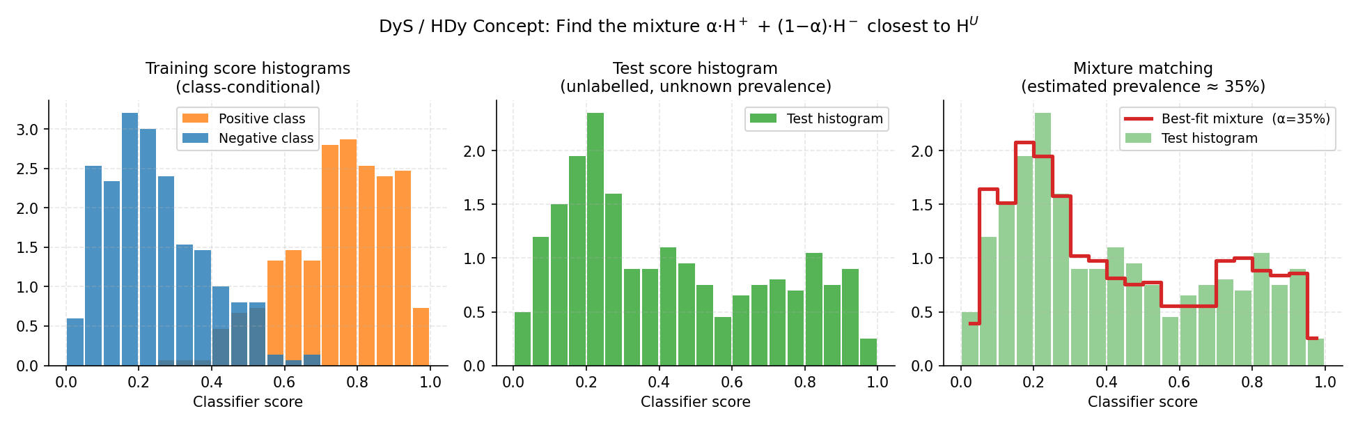
Left: class-conditional score histograms learned from training data. Centre: test score histogram (unlabelled — unknown prevalence). Right: DyS searches for the mixture proportion α that makes α·H⁺ + (1−α)·H⁻ (red step line) match the test histogram (green bars) as closely as possible.

2.7.1.3. Examples

Basic binary usage:

from mlquantify.matching import DyS
from sklearn.linear_model import LogisticRegression
from sklearn.datasets import make_classification
from sklearn.model_selection import train_test_split

X, y = make_classification(n_samples=1000, weights=[0.8, 0.2],
                           random_state=42)
X_train, X_test, y_train, y_test = train_test_split(
    X, y, test_size=0.3, random_state=42)

q = DyS(estimator=LogisticRegression())
q.fit(X_train, y_train)
print(q.predict(X_test))
# {0: 0.79, 1: 0.21}

Customising bins and distance:

import numpy as np
from mlquantify.matching import DyS
from sklearn.linear_model import LogisticRegression

q = DyS(
    estimator=LogisticRegression(),
    bins_size=np.arange(2, 32, 2),   # sweep 2,4,6,...,30 bins
    distance='hellinger',
    bin_strategy='median',           # median across all bin sizes
    laplace_smoothing=True,
)
q.fit(X_train, y_train)
print(q.predict(X_test))

Using aggregate with pre-computed scores:

import numpy as np
from mlquantify.matching import DyS
from sklearn.linear_model import LogisticRegression

clf = LogisticRegression().fit(X_train, y_train)
# Positive-class scores (column 1)
train_scores = clf.predict_proba(X_train)[:, 1]
test_scores  = clf.predict_proba(X_test)[:, 1]

q = DyS(clf)
q.fit(X_train, y_train)
print(q.aggregate(test_scores, train_scores, y_train))

---

2.7.1.4. HDy — Hellinger Distance y-Similarity

HDy (González-Castro et al., 2013) is a specific instantiation of the DyS framework that sweeps over multiple bin sizes (\(10, 20, \ldots, 110\) by default) and returns the median prevalence across all bin sizes. It uses the Hellinger distance as the dissimilarity.

Why it exists: HDy was the original paper that introduced the idea of comparing score histograms for quantification. The multi-bin median strategy reduces sensitivity to the bin count hyperparameter, making HDy robust without tuning.

2.7.1.5. Parameters

Same structure as DyS. Key defaults:

• distance='hellinger'

• bin_strategy='median'

• bins_size=np.linspace(10, 110, 11, dtype=int)

from mlquantify.matching import HDy
from sklearn.linear_model import LogisticRegression

q = HDy(estimator=LogisticRegression())
q.fit(X_train, y_train)
print(q.predict(X_test))

---

2.7.1.6. HDx — Hellinger Distance x-Similarity (classifier-free)

HDx (González-Castro et al., 2013) compares class-conditional feature histograms directly, without using a classifier. For each feature, it builds a histogram for each class; the mixture of feature histograms that best matches the test histogram gives the prevalence estimate.

Why it exists: HDx is a non-aggregative histogram method — it does not need a classifier at all. It is useful when no reliable classifier is available, or as a sanity check. Performance is generally below HDy/DyS (which use a classifier’s summary score), but it is a zero-cost baseline.

2.7.1.7. Parameters

Parameter	Default	Explanation
bins_size	None	Array of bin counts to sweep (default: [2,4,6,...,20,30]).
strategy	'ovr'	Multiclass decomposition.

from mlquantify.matching import HDx

q = HDx()
q.fit(X_train, y_train)
print(q.predict(X_test))
# No classifier needed

---

2.7.1.8. SMM — Score Mixture Model

SMM extends DyS to use a more flexible representation of the score distribution. Parameters match DyS.

---

2.7.2. Density Methods — KDEy

KDE-based methods replace histograms with smooth kernel density estimates (KDE), avoiding bin-count sensitivity while still matching distributions.

2.7.2.1. KDEy-HD, KDEy-CS, KDEy-ML

The three KDEy variants (Moreo et al., 2024) share the same architecture: they build a KDE over classifier posteriors on the training data (for each class) and minimise a dissimilarity to the test KDE at prediction time. They differ in the dissimilarity used:

• KDEyHD — Hellinger distance between KDEs.

• KDEyCS — squared cosine distance between KDEs.

• KDEyML — maximises the mixture log-likelihood (equivalent to minimising negative log-likelihood).

Why they exist: KDEy methods are natively multiclass (unlike DyS/HDy) and avoid the histogram bin-count hyperparameter. Moreo et al. (2024) showed they are state-of-the-art for multiclass quantification.

2.7.2.2. Parameters

Parameter	Default	Explanation
estimator	None	Probabilistic classifier.
bandwidth	0.1	KDE bandwidth (smoothing). Smaller values give sharper densities (more variance), larger values smooth them out (more bias). Use cross-validation to tune: try [0.01, 0.05, 0.1, 0.2, 0.5].
kernel	'gaussian'	KDE kernel type. 'gaussian' works well for probability scores in \([0,1]\). Matches sklearn.neighbors.KernelDensity options.
solver	'slsqp'	Optimisation solver for the simplex-constrained mixture problem.
cv	None	Cross-validation folds.
stratified	True	Stratified folds.

2.7.2.3. Examples

Binary with KDEyHD:

from mlquantify.matching import KDEyHD
from sklearn.linear_model import LogisticRegression

q = KDEyHD(estimator=LogisticRegression(), bandwidth=0.1)
q.fit(X_train, y_train)
print(q.predict(X_test))

Multiclass with KDEyML (best accuracy):

from mlquantify.matching import KDEyML
from sklearn.linear_model import LogisticRegression
from sklearn.datasets import make_classification

X, y = make_classification(n_samples=800, n_classes=4,
                           n_informative=6, n_redundant=0,
                           random_state=42)
X_train, X_test = X[:600], X[600:]
y_train = y[:600]

q = KDEyML(LogisticRegression(), bandwidth=0.05)
q.fit(X_train, y_train)
print(q.predict(X_test))

Tuning bandwidth with grid search:

from mlquantify.model_selection import GridSearchQ
from mlquantify.matching import KDEyHD
from mlquantify.model_selection import APP
from mlquantify.metrics import MAE
from sklearn.linear_model import LogisticRegression

protocol = APP(batch_size=100, n_prevalences=21, repeats=5)
gs = GridSearchQ(
    quantifier=KDEyHD(LogisticRegression()),
    param_grid={'bandwidth': [0.01, 0.05, 0.1, 0.2, 0.5]},
    protocol=protocol,
    error=MAE,
)
gs.fit(X_train, y_train)
print(gs.best_params_)

Tip

Use KDEyML for multiclass problems — it is consistently the most accurate KDE variant in Moreo et al. (2024)’s benchmark. Use KDEyHD for binary problems if you want a fast alternative to DyS.

---

2.7.3. Kernel Methods — MMD

MMD_RKHS (Maximum Mean Discrepancy in Reproducing Kernel Hilbert Space) matches class-conditional kernel mean embeddings of the raw feature vectors, rather than classifier scores. It directly computes the kernel mean of each class in feature space and finds the mixture that minimises the MMD to the test kernel mean.

Why it exists: MMD_RKHS is a non-aggregative method (no classifier needed) that works directly on the feature space via a kernel trick. It is useful when features are naturally compared with a kernel (e.g. strings, graphs, or dense embeddings). Iyer et al. (2014) showed strong convergence guarantees for kernel quantification.

2.7.3.1. Parameters

Parameter	Default	Explanation
kernel	'rbf'	Kernel function for computing the RKHS mean embedding. Options: 'rbf', 'linear', 'poly', 'sigmoid', 'cosine'. 'rbf' works well for continuous features.
gamma	None	RBF/poly/sigmoid bandwidth. None uses 1/n_features. Tune this if features are on very different scales (consider normalising first).
degree	3	Polynomial degree for 'poly' kernel.
coef0	0.0	Independent term for poly/sigmoid kernels.
solver	'slsqp'	Optimisation solver.

from mlquantify.matching import MMD_RKHS

q = MMD_RKHS(kernel='rbf', gamma=0.1)
q.fit(X_train, y_train)      # No classifier — works on raw features
print(q.predict(X_test))

---

2.7.4. Score Methods — SORD

SORD (Score-based Optimal Ranking Distribution) estimates prevalence by comparing the ranked order of classifier scores between the test set and the mixture of class-conditional training scores, using an earth-mover-style distance.

Why it exists: SORD operates on the continuous score values without discretisation (no bins needed) and without density estimation. It is fast, parameter-free (beyond the classifier), and competitive with histogram methods.

from mlquantify.matching import SORD
from sklearn.linear_model import LogisticRegression

q = SORD(estimator=LogisticRegression())
q.fit(X_train, y_train)
print(q.predict(X_test))

---

2.7.5. Choosing a Distribution Matching Method

Method	Multiclass	Needs clf	Key hyperparameter	Best for
DyS	✗ (OvR)	✓	bins_size, distance	Binary; strong with median-sweep bins.
HDy	✗ (OvR)	✓	bins_size	Binary; tuning-free median-sweep baseline.
HDx	✗ (OvR)	✗	bins_size	No classifier available; sanity check.
KDEyHD	✓	✓	bandwidth	Binary & multiclass; smooth density matching.
KDEyML	✓	✓	bandwidth	Multiclass; best overall accuracy.
MMD_RKHS	✓	✗	kernel, gamma	Kernel-based features; no classifier needed.
SORD	✗ (OvR)	✓	None	Binary; parameter-free, fast.

Practical recommendation:

• For binary problems: DyS or MS (threshold-adjustment) are strong.

• For multiclass problems: KDEyML is the recommended starting point.

• When no classifier is available: HDx or MMD_RKHS.

• For a parameter-free binary option: SORD.

See also

Likelihood-Based Quantification for EMQ, which is often as good as or better than DM methods under pure prior probability shift.

Distribution Matching (DM) methods estimate prevalences by matching the test distribution to a mixture of class-conditional distributions learned on the training data. In practice, the matching strategy depends on how distributions are represented.

The matching module is organized around four representation families:

• Histogram: histogram-based matching (DyS, HDy, SMM).

• Density: KDE-based matching over the probability simplex (KDEy variants).

• Kernel: kernel mean matching in RKHS (MMD_RKHS).

• Scores: matching directly on score samples (SORD).

Mathematical details - Mixture Formulation

The observed distribution in the test set is approximated as:

\[D_U \approx \hat{p} \cdot D_+ + (1 - \hat{p}) \cdot D_-\]

DM methods search for the mixture parameter \(\hat{p}\) that minimizes a chosen dissimilarity between the test distribution and the mixture.

References

[1]

Forman, G. (2008). Quantifying counts and costs via classification. Data Mining and Knowledge Discovery, 17(2), 164-206. https://doi.org/10.1007/s10618-008-0097-y

2.7.6. Histogram

Histogram-based DM builds class-conditional histograms of posterior scores and fits the test histogram as a mixture of those class histograms. These methods are binary-first and default to one-vs-rest for multiclass settings.

2.7.6.1. DyS: Distribution y-Similarity Framework

DyS is a generic framework that formalizes histogram-based matching. It selects the prevalence \(\alpha\) that minimizes a dissimilarity between the test score histogram and the mixture of training histograms [2].

Mathematical details - DyS Optimization

\[\hat{p}^{DyS}(\oplus) = \alpha^* = \operatorname*{arg\,min}_{0 \le \alpha \le 1} \{ DS(\alpha f_{L^{\oplus}} + (1-\alpha) f_{L^{\ominus}}, f_U) \}\]

2.7.6.2. HDy: Hellinger Distance y-Similarity

HDy is a popular instance of DyS that uses the Hellinger distance over histograms of posterior probabilities.

from mlquantify.matching import HDy
from sklearn.ensemble import RandomForestClassifier

q = HDy(estimator=RandomForestClassifier(), bins=10)
q.fit(X_train, y_train)
q.predict(X_test)

Mathematical details - HDy Bin Adjustment

\[\frac{|D'_i|}{|D'|} = \frac{|D^+_i|}{|D^+|} \cdot \hat{p} + \frac{|D^-_i|}{|D^-|} \cdot (1 - \hat{p})\]

2.7.6.3. SMM: Sample Mean Matching

SMM replaces histograms with a single statistic: the mean score. It solves the mixture matching problem in closed form and is equivalent to PACC [4].

Mathematical details - SMM Closed Form

\[\alpha = \frac{\mu[S_U] - \mu[S_{\ominus}]}{\mu[S_{\oplus}] - \mu[S_{\ominus}]}\]

(Source code, png, hires.png, pdf)

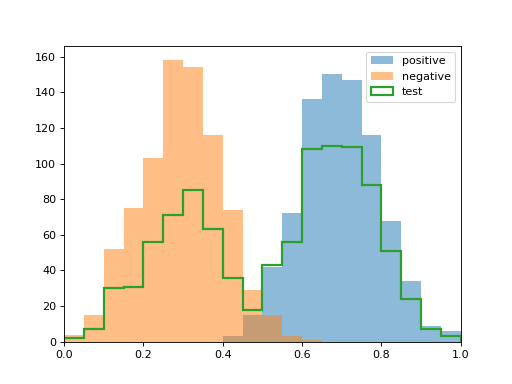
Histogram mixtures used by DyS/HDy-like methods.

References

[2]

Maletzke, A., dos Reis, D., Cherman, E., & Batista, G. (2019). DyS: A Framework for Mixture Models in Quantification. AAAI.

[3]

González-Castro, V., Alaiz-Rodríguez, R., & Alegre, E. (2013). Class distribution estimation based on the Hellinger distance. Information Sciences, 218, 146-164. https://doi.org/10.1016/j.ins.2012.05.028

[4]

Hassan, W., Maletzke, A., & Batista, G. (2020). Accurately quantifying a billion instances per second. IEEE DSAA.

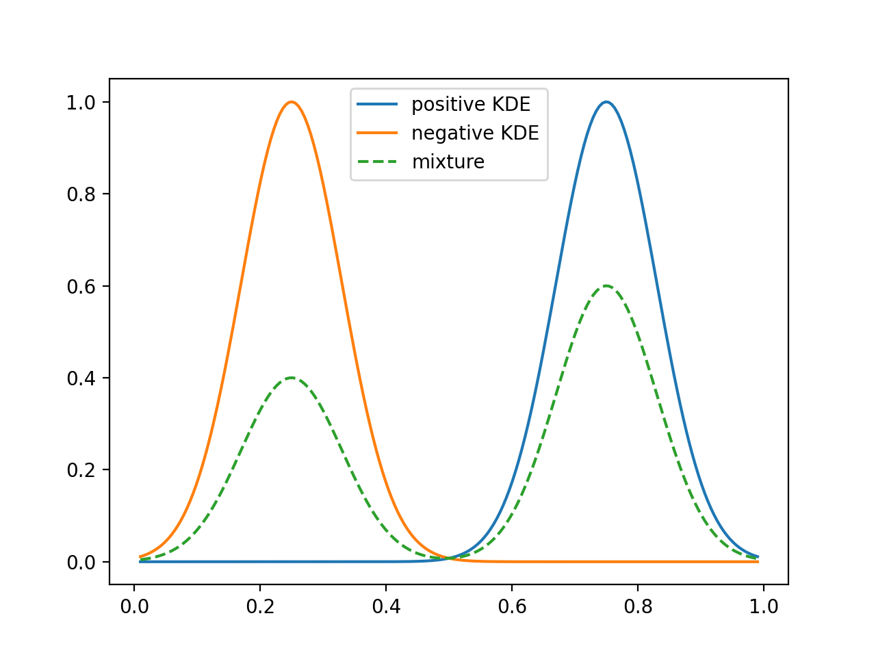
2.7.7. Density

2.7.7.1. KDEy: Kernel Density Estimation y-Similarity

KDEy is a multi-class DM approach that replaces histograms with continuous densities over the probability simplex, allowing it to model inter-class interactions and avoid binning artifacts [5].

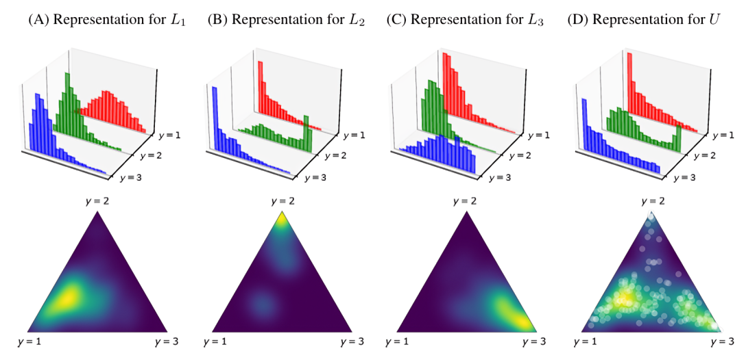
Illustration of KDEy modeling class-conditional densities on the probability simplex.

2.7.7.2. KDEy-ML (Maximum Likelihood)

The KDEyML class maximizes the likelihood of the test scores under the mixture of KDE class-conditional densities.

Mathematical details - KDEy-ML Optimization

\[\hat{\alpha} = \operatorname*{arg\,min}_{\alpha \in \Delta^{n-1}} \left( - \sum_{x \in U} \log \left( \sum_{i=1}^{n} \alpha_i \cdot p_{\tilde{L}_i}(x) \right) \right)\]

2.7.7.3. KDEy-HD (Hellinger Distance)

The KDEyHD class minimizes the Hellinger distance between the test KDE and the mixture of class-conditional KDEs using Monte Carlo approximation.

2.7.7.4. KDEy-CS (Cauchy-Schwarz)

The KDEyCS class minimizes the Cauchy-Schwarz divergence with a closed form that leverages kernel Gram matrices.

(Source code, png, hires.png, pdf)

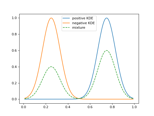
KDE-based density matching over the simplex (illustrative).

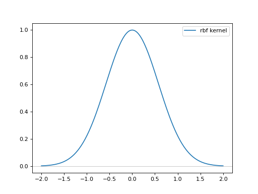
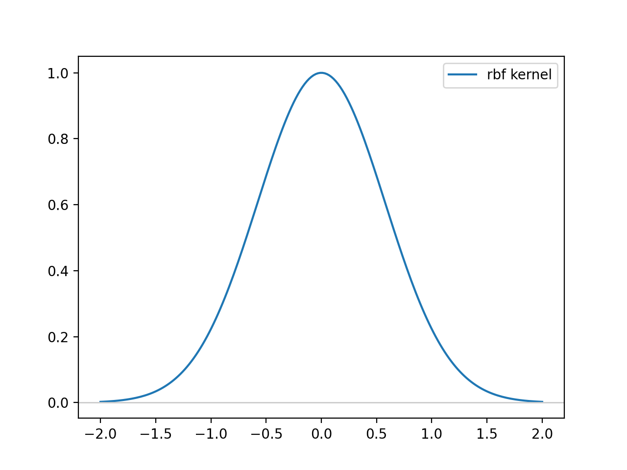
2.7.8. Kernel

Kernel matching minimizes the distance between the kernel mean embedding of the test sample and the mixture of class-conditional kernel mean embeddings. The MatchingKernelQuantifier base class implements this strategy and the MMD_RKHS quantifier provides the standard RKHS formulation [6].

(Source code, png, hires.png, pdf)

Kernel similarities used for mean matching.

References

[6]

Zhang, K., Schölkopf, B., Muandet, K., & Wang, Z. (2013). Domain Adaptation under Target and Conditional Shift. ICML.

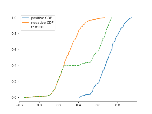
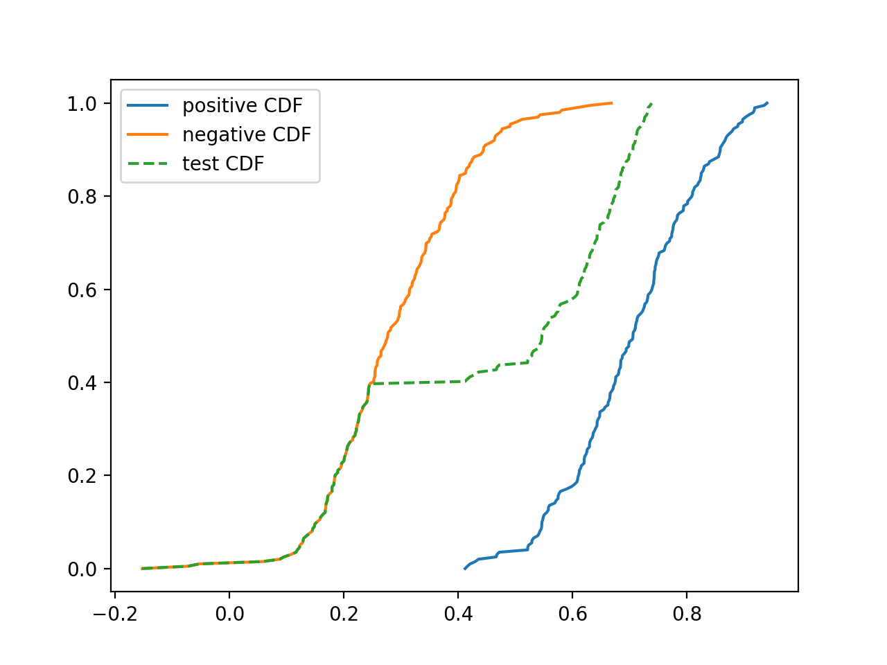
2.7.9. Scores

Score-based matching works directly on the score samples rather than binned histograms. The SORD quantifier minimizes a cumulative distance between the test score distribution and the weighted mixture of train scores.

(Source code, png, hires.png, pdf)

Sample-based matching with cumulative score distances.

References

[5]

Moreo, A., González, P., & del Coz, J. J. (2024). Kernel Density Estimation for Multiclass Quantification. http://arxiv.org/abs/2401.00490

[7]

Maletzke, A., dos Reis, D., Hassan, W., & Batista, G. (2021). Accurately Quantifying under Score Variability.