5.1. Protocols for Quantification#

Evaluating a quantifier on a single test set is misleading — the test prevalence is fixed, so you only see performance at one operating point. Quantification protocols address this by generating many test batches with varying prevalences from the same data, giving a fuller picture of method behaviour across the entire prevalence spectrum.

Why protocols matter

A quantifier that looks excellent at 50/50 prevalence may fail badly at 5/95. Forman (2005) noted that the choice of evaluation protocol is as important as the choice of method. Standard practice in quantification research is to evaluate across a grid of prevalences (APP) and report the mean error over all samples.

5.1.1. Quick evaluation with `apply_protocol`#

apply_protocol runs the whole evaluation loop in a single call — the protocol analogue of scikit-learn’s cross_validate. It fits the quantifier, samples the test batches with the chosen protocol, predicts each one, and returns the true and predicted prevalences together with one score array per metric:

from mlquantify.model_selection import apply_protocol
from mlquantify.likelihood import EMQ
from sklearn.linear_model import LogisticRegression
from sklearn.datasets import make_classification

X, y = make_classification(n_samples=2000, weights=[0.7, 0.3], random_state=42)

results = apply_protocol(
    EMQ(LogisticRegression()), X, y,
    protocol="app",           # 'app' | 'npp' | 'upp' | 'ppp'
    scoring=["mae", "nmd"],   # one metric name, a callable, or a list
    n_prevalences=21,
    batch_size=100,
    test_size=0.5,            # held-out pool the protocol samples from
    random_state=42,
)

print("samples:", results["n_batches"])
print("MAE:", results["MAE"].mean(), "NMD:", results["NMD"].mean())
# results["true_prevalences"], results["predicted_prevalences"] -> (n_samples, n_classes)

By default a copy of the quantifier is trained on 1 - test_size of the data and evaluated on the rest. Pass fit=False to evaluate an already-fitted quantifier, return_estimator=True to get the trained model back, or a BaseProtocol instance as protocol for full control. The sections below document the underlying protocols, which you can also drive manually.

5.1.2. APP — Artificial Prevalence Protocol #

APP is the most widely used evaluation protocol. By default it draws samples from the test set at each prevalence in a uniform grid \(\{0, \frac{1}{n-1}, \frac{2}{n-1}, \ldots, 1\}\) for the positive class, repeating each prevalence repeats times.

Why it is standard: APP ensures every method is evaluated at many prevalence values, not just the natural one. It exposes systematic biases (e.g. methods that only work near 50/50) and gives a fair cross-method comparison. González et al. (2017) review papers routinely use APP as the evaluation backbone.

Choosing how prevalences are produced. The strategy parameter selects how the prevalence vectors are drawn over the simplex. 'grid' is the classic systematic sweep; the other strategies sample the simplex and scale to many classes without the grid’s combinatorial blow-up. UPP is simply APP with a sampling strategy pinned on.

5.1.2.1. Parameters #

Parameter	Default	Explanation
`batch_size`	required	Number of instances per test sample. Larger batches give more stable prevalence estimates but require a larger test set. A typical choice is 100–500.
`n_prevalences`	`21`	Number of equally-spaced prevalence points from `min_prev` to `max_prev`. `21` gives a step of 0.05 (i.e. 0%, 5%, 10%, …, 100%).
`repeats`	`10`	How many independent samples to draw at each prevalence level. More repeats reduce variance in the average error estimate. Use ≥ 5 for reliable results.
`min_prev`	`0.0`	Minimum positive class prevalence in the grid. Leave at 0 to include the all-negative case.
`max_prev`	`1.0`	Maximum positive class prevalence. Leave at 1 to include the all-positive case.
`strategy`	`'grid'`	How prevalence vectors are generated over the simplex: `'grid'` — a regular lattice of evenly-spaced prevalences from `min_prev` to `max_prev` (the classic APP). Deterministic and systematic, but the number of points grows combinatorially (\(O(n^{k-1})\) for `k` classes), so it is best for binary or low-class-count problems. `'kraemer'` — the Kraemer method for uniform sampling over the simplex. Every prevalence combination is equally likely and the cost is independent of the number of classes, ideal for multiclass. `'uniform'` — uniform sampling via the flat Dirichlet \(\mathrm{Dir}(\mathbf{1})\). Statistically equivalent to `'kraemer'` but produced through the Dirichlet route; it is exactly `'dirichlet'` with `dirichlet_alpha=1`. `'dirichlet'` — sampling from a Dirichlet whose concentration is set by `dirichlet_alpha`, letting you bias the prevalences (see below).
`dirichlet_alpha`	`1.0`	Concentration for `strategy='dirichlet'`. A scalar is broadcast to a symmetric Dirichlet; an array of length `n_classes` sets a per-class concentration. `alpha > 1` favours balanced prevalences near the centre of the simplex; `alpha < 1` favours extreme, one-class-dominant prevalences near the corners; `alpha = 1` is uniform. Ignored by the other strategies.
`random_state`	`None`	Seed for reproducible sampling.

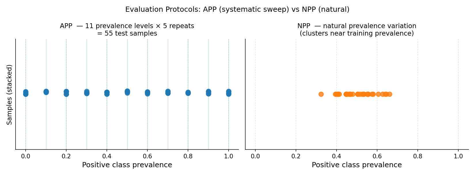
APP vs NPP protocol comparison — Left: APP generates test samples at every point on a regular prevalence grid (blue dots), giving systematic coverage from 0% to 100% positive class. Right: NPP draws random sub-samples that cluster near the natural training prevalence (~50%), providing realistic but narrower coverage.#

5.1.2.2. Examples #

Standard evaluation loop:

from mlquantify.model_selection import APP
from mlquantify.metrics import MAE
from mlquantify.utils import get_prev_from_labels
from mlquantify.likelihood import EMQ
from sklearn.linear_model import LogisticRegression
from sklearn.datasets import make_classification
from sklearn.model_selection import train_test_split
import numpy as np

X, y = make_classification(n_samples=2000, weights=[0.7, 0.3],
                           random_state=42)
X_train, X_test, y_train, y_test = train_test_split(
    X, y, test_size=0.5, random_state=42)

q = EMQ(LogisticRegression())
q.fit(X_train, y_train)

protocol = APP(batch_size=100, n_prevalences=21, repeats=10,
               random_state=42)
errors = []
for idx in protocol.split(X_test, y_test):
    X_sample, y_sample = X_test[idx], y_test[idx]
    true_prev = get_prev_from_labels(y_sample)
    pred_prev = q.predict(X_sample)
    errors.append(MAE(true_prev, pred_prev))

print(f"Mean MAE over {len(errors)} samples: {np.mean(errors):.4f}")

Comparing multiple quantifiers:

from mlquantify.counting import CC, PCC
from mlquantify.likelihood import EMQ
from mlquantify.matching import DyS
from sklearn.linear_model import LogisticRegression

quantifiers = {
    'CC':  CC(LogisticRegression()),
    'PCC': PCC(LogisticRegression()),
    'EMQ': EMQ(LogisticRegression()),
    'DyS': DyS(LogisticRegression()),
}

for name, q in quantifiers.items():
    q.fit(X_train, y_train)

protocol = APP(batch_size=100, n_prevalences=21, repeats=10,
               random_state=42)

results = {name: [] for name in quantifiers}
for idx in protocol.split(X_test, y_test):
    X_s, y_s = X_test[idx], y_test[idx]
    true_prev = get_prev_from_labels(y_s)
    for name, q in quantifiers.items():
        results[name].append(MAE(true_prev, q.predict(X_s)))

for name, errs in results.items():
    print(f"{name:5s}  MAE={np.mean(errs):.4f}")

5.1.3. NPP — Natural Prevalence Protocol #

NPP draws random sub-samples from the test set without altering the natural class distribution. Each sample has a slightly different prevalence due to random variation, but no artificial manipulation is performed.

Why it exists: NPP evaluates quantifiers under real prevalence variation — how they perform when deployed on random sub-populations drawn from the same underlying distribution as the test set. It is less controlled than APP but more realistic.

Limitation: Because NPP cannot produce extreme prevalences (e.g. 2% positive) without a very large test set, it gives a narrower view of method behaviour than APP.

5.1.3.1. Parameters #

Parameter	Default	Explanation
`batch_size`	required	Size of each random sub-sample.
`n_samples`	`100`	Number of random sub-samples to draw.
`random_state`	`None`	Seed for reproducibility.

from mlquantify.model_selection import NPP
from mlquantify.utils import get_prev_from_labels

protocol = NPP(batch_size=100, n_samples=50, random_state=42)
for idx in protocol.split(X_test, y_test):
    X_s, y_s = X_test[idx], y_test[idx]
    true_prev = get_prev_from_labels(y_s)
    pred_prev = q.predict(X_s)

5.1.4. UPP — Uniform Prevalence Protocol #

UPP samples prevalence vectors uniformly from the probability simplex. It is exactly APP with the simplex sampling strategy pinned on ('kraemer' by default). For binary problems it is similar to APP, but for multiclass problems it avoids the combinatorial explosion of sweeping all class-prevalence combinations independently.

Why it exists: For \(k\) classes, a grid approach like APP grows as \(O(n^{k-1})\) which quickly becomes intractable. UPP samples \(n\) random vectors from the simplex, covering the multiclass prevalence space efficiently without a rigid grid. Maletzke et al. (2020) recommend UPP for multiclass evaluation.

5.1.4.1. Parameters #

Parameter	Default	Explanation
`batch_size`	required	Size of each sample.
`n_prevalences`	`100`	Number of prevalence vectors to sample from the simplex.
`strategy`	`'kraemer'`	Simplex sampling strategy, forwarded to `APP` (`'grid'` is not meaningful here): `'kraemer'` — Kraemer uniform sampling over the simplex. All prevalence combinations are equally likely; cost independent of the number of classes. `'uniform'` — uniform sampling via the flat Dirichlet (\(\text{Dir}(\mathbf{1})\)); equivalent uniform coverage through the Dirichlet route. `'dirichlet'` — Dirichlet sampling biased by `dirichlet_alpha` (see `APP`).
`dirichlet_alpha`	`1.0`	Concentration used when `strategy='dirichlet'`; see `APP`.
`algorithm`	(deprecated)	Deprecated alias for `strategy`; kept for backward compatibility.
`min_prev`	`0.0`	Minimum per-class prevalence. Raise (e.g. to `0.01`) to avoid near-zero classes that are hard to sample from small datasets.
`max_prev`	`1.0`	Maximum per-class prevalence.
`random_state`	`None`	Seed.

from mlquantify.model_selection import UPP
from mlquantify.utils import get_prev_from_labels
from sklearn.datasets import make_classification

X, y = make_classification(n_samples=2000, n_classes=4,
                           n_informative=6, n_redundant=0,
                           random_state=42)
X_train, X_test = X[:1500], X[1500:]
y_train, y_test = y[:1500], y[1500:]

protocol = UPP(batch_size=100, n_prevalences=200, strategy='uniform',
               random_state=42)
errors = []
for idx in protocol.split(X_test, y_test):
    X_s, y_s = X_test[idx], y_test[idx]
    true_prev = get_prev_from_labels(y_s)
    pred_prev = q.predict(X_s)
    errors.append(MAE(true_prev, pred_prev))

5.1.5. PPP — Personalized Prevalence Protocol #

PPP generates samples at class prevalences you specify explicitly, for targeted evaluation at exact operating points (where APP and UPP sweep the prevalences for you). Pass a list of prevalence vectors; in the binary case a single float is read as the positive-class prevalence.

5.1.5.1. Parameters #

Parameter	Default	Explanation
`batch_size`	required	Size of each sample.
`prevalences`	required	List of target prevalence vectors (or floats for binary problems).
`repeats`	`1`	Number of samples drawn per target prevalence.
`random_state`	`None`	Seed for reproducibility.

from mlquantify.model_selection import PPP
from mlquantify.utils import get_prev_from_labels

protocol = PPP(batch_size=100,
               prevalences=[[0.1, 0.9], [0.5, 0.5], [0.9, 0.1]],
               random_state=42)
for idx in protocol.split(X_test, y_test):
    X_s, y_s = X_test[idx], y_test[idx]
    true_prev = get_prev_from_labels(y_s)
    pred_prev = q.predict(X_s)

5.1.6. Choosing a Protocol #

Protocol	Problem type	Use when
APP	Binary	Default for binary problems. Systematic sweep; standard in quantification research. Forman (2005) introduced the concept.
NPP	Binary / multiclass	You want realistic evaluation under natural prevalence variation.
UPP (uniform)	Multiclass	Default for multiclass. Efficient random coverage of the simplex.
UPP (kraemer)	Multiclass	You need a deterministic grid equivalent to APP for multiclass.
PPP	Binary / multiclass	You want to evaluate at specific, hand-picked prevalences.

Tip

For most workflows, reach for apply_protocol rather than writing the loop by hand — it accepts the same protocol choice and returns the scores directly.

Tip

Always fix random_state in protocols when comparing methods so that all quantifiers are evaluated on exactly the same test samples.

References

Forman, G. (2008). Quantifying Counts and Costs via Classification. Data Mining and Knowledge Discovery, 17(2), 164–206.
González, P., Castaño, A., Chawla, N. V., & del Coz, J. J. (2017). A Review on Quantification Learning. ACM Computing Surveys, 50(5), 1–40.
Esuli, A., Fabris, A., Moreo, A., & Sebastiani, F. (2023). Learning to Quantify. The Information Retrieval Series, Springer.